
Supervised machine learning models
Logistic Regression
Logistic regression is used when you have a classification problem. This means that your target variable (a.k.a. the variable you are interested in predicting) is made up of categories. These categories could be yes/no, or something like a number between 1 and 10 representing customer satisfaction.
The logistic regression model uses an equation to create a curve with your data and then uses this curve to predict the outcome of a new observation.
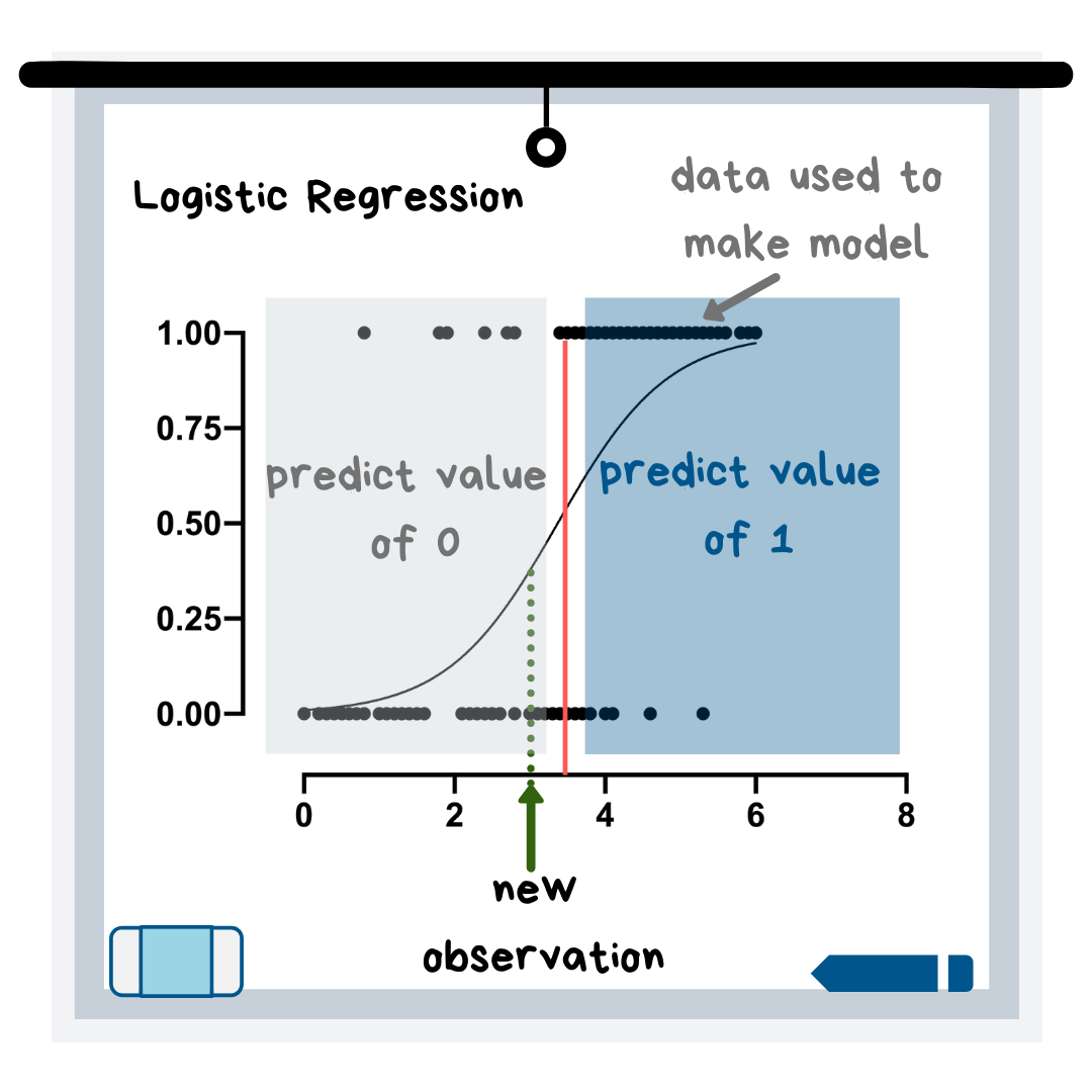
In the graphic above, the new observation would get a prediction of 0 because it falls on the left side of the curve. If you look at the data this curve is based on, it makes sense because, in the “predict a value of 0” region of the graph, the majority of the data points have a y-value of 0.
Linear Regression
Linear regression is often one of the first machine learning models that people learn. This is because its algorithm (i.e. the equation behind the scenes) is relatively easy to understand when using just one x-variable — it is just making a best-fit line, a concept taught in elementary school. This best-fit line is then used to make predictions about new data points (see illustration).
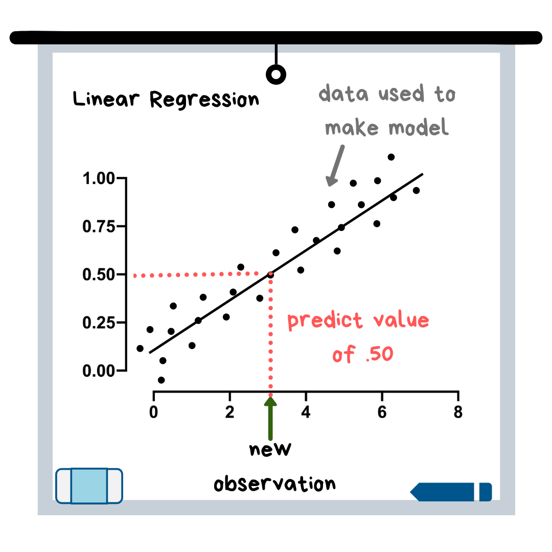
Linear Regression is similar to logistic regression, but it is used when your target variable is continuous, which means it can take on essentially any numerical value. In fact, any model with a continuous target variable can be categorized as “regression.” An example of a continuous variable would be the selling price of a house.
Linear regression is also very interpretable. The model equation contains coefficients for each variable, and these coefficients indicate how much the target variable changes for each small change in the independent variable (the x-variable). With the house prices example, this means that you could look at your regression equation and say something like “oh, this tells me that for every increase in 1ft² of house size (the x-variable), the selling price (the target variable) increases by $25.”
K Nearest Neighbors (KNN)
This model can be used for either classification or regression! The name “K Nearest Neighbors” is not intended to be confusing. The model first plots out all of the data. The “K” part of the title refers to the number of closest neighboring data points that the model looks at to determine what the prediction value should be (see illustration below). You, as the future data scientist, get to choose K and you can play around with the values to see which one gives the best predictions.
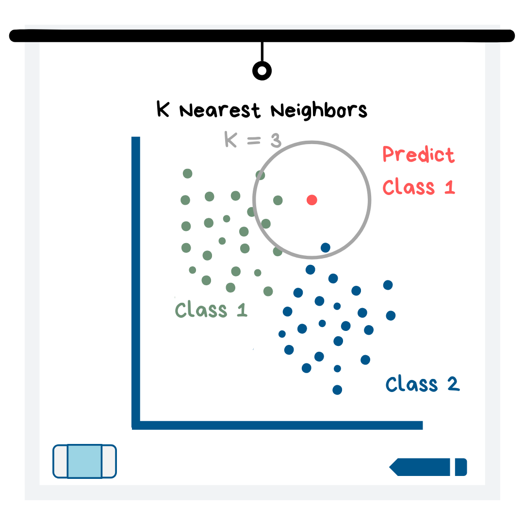
All of the data points that are in the K=__ circle get a “vote” on what the target variable value should be for this new data point. Whichever value receives the most votes is the value that KNN predicts for the new data point. In the illustration above, 2 of the nearest neighbors are class 1, while 1 of the neighbors is class 2. Thus, the model would predict class 1 for this data point. If the model is trying to predict a numerical value instead of a category, then all of the “votes” are numerical values that are averaged to get a prediction.
Support Vector Machines (SVMs)
Support Vector Machines work by establishing a boundary between data points, where the majority of one class falls on one side of the boundary (a.k.a. line in the 2D case) and the majority of the other class falls on the other side.
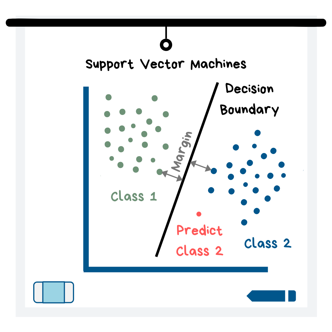
The way it works is the machine seeks to find the boundary with the largest margin. The margin is defined as the distance between the nearest point of each class and the boundary (see illustration). New data points are then plotted and put into a class depending on which side of the boundary they fall on.
My explanation of this model is for the classification case, but you can also use SVMs for regression!
Decision trees & random forests
I already explained these in a previous article — check it out here (decision trees and random forests are near the end).