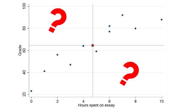
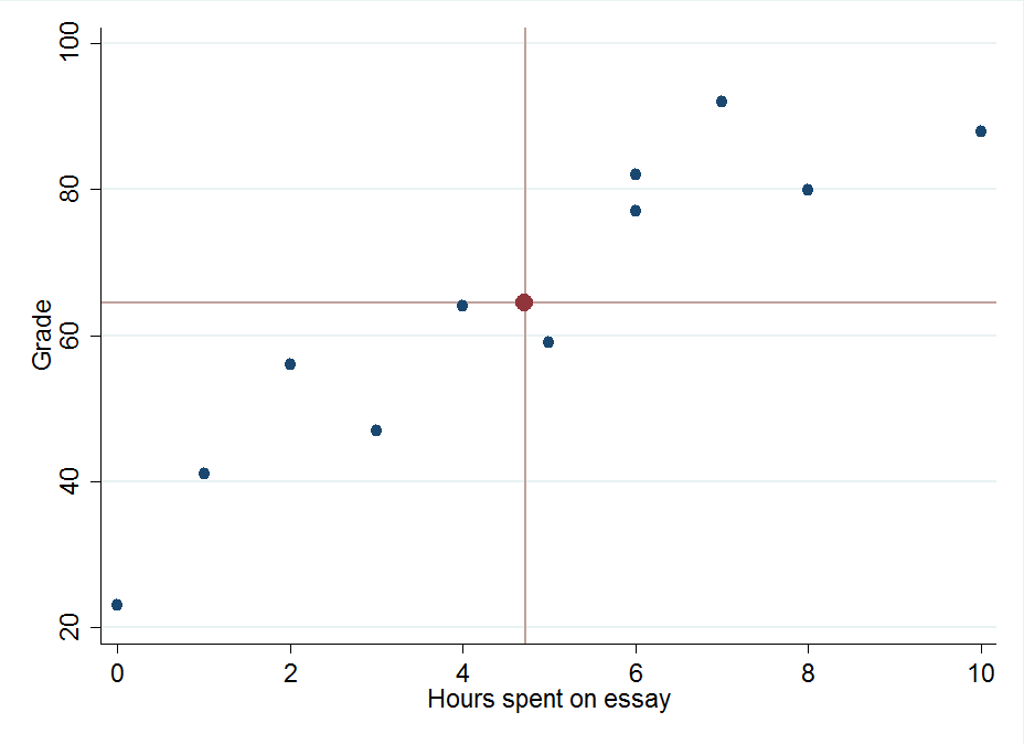
When calculating least squares regressions by hand, the first step is to find the means of the dependent and independent variables. We do this because of an interesting quirk within linear regression lines – the line will always cross the point where the two means intersect. We can think of this as an anchor point, as we know that the regression line in our test score data will always cross (4.72, 64.45).
The second step is to calculate the difference between each value and the mean value for
both the dependent and the independent variable. In this case this means we subtract 64.45
from each test score and 4.72 from each time data point. Additionally,
we want to find the product of multiplying these two differences together.

You should notice that as some scores are lower than the mean score, we end up with negative values. By squaring these differences, we end up with a standardized measure of deviation from the mean regardless of whether the values are more or less than the mean.
Let’s remind ourselves of the equation we need to calculate b.
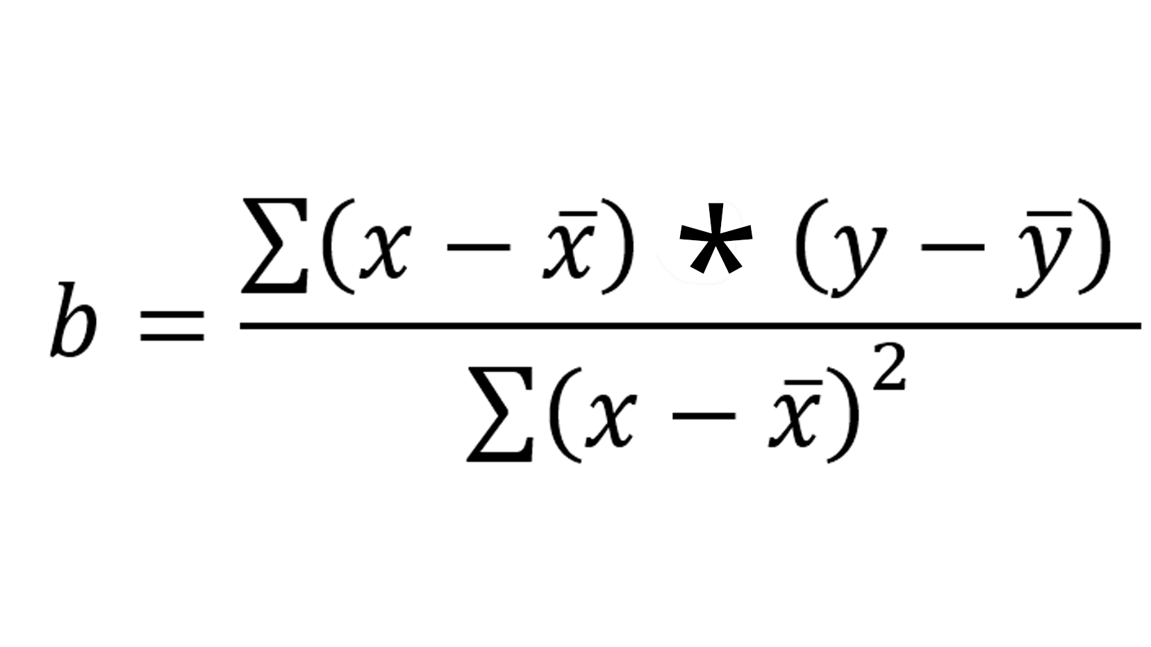
The symbol sigma (∑) tells us we need to add all the relevant values together.
If we do this for the table above, we get the following results:
∑(x-x ̅ ) * (y-y ̅ ) = 611.36
And
∑(x-x ̅ ) ^2 = 94.18
Slotting in the information from the above table into a calculator allows us to calculate b, which is step one of two to unlock the predictive power of our shiny new model:

The final step is to calculate the intercept, which we can do using the initial regression equation with the values of test score and time spent set as their respective means, along with our newly calculated coefficient.
64.45= a + 6.49*4.72
We can then solve this for a:
64.45 = a + 30.63
a = 64.45 – 30.63
a = 30.18
Now we have all the information needed for our equation and are free to slot in values as we see fit. If we wanted to know the predicted grade of someone who spends 2.35 hours on their essay, all we need to do is swap that in for X.
y=30.18 + 6.49 * X
y = 30.18 + (6.49 * 2.35)
y = 45.43
Drawing a Least Squares Regression Line by Hand
If we wanted to draw a line of best fit, we could calculate the estimated grade for a series of time values and then connect them with a ruler. As we mentioned before, this line should cross the means of both the time spent on the essay and the mean grade received.
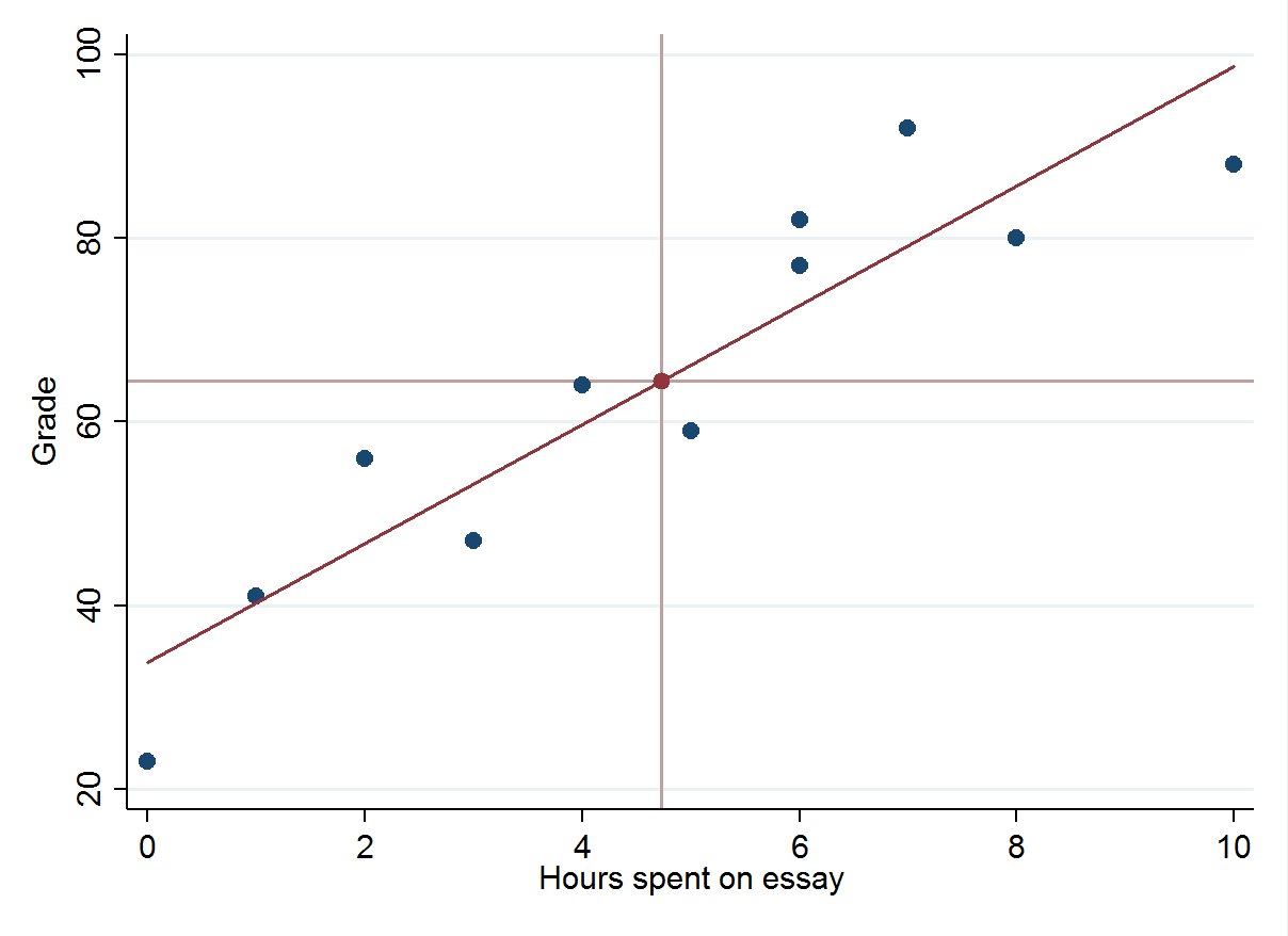
And there we have it! A perfect* predictive model that will make our teachers’ lives a lot easier.


