Introductory Guide To PyTorch Using A Linear Regression Problem

Let’s look at the line by line explanation below:

1. Defining a class called LinearRegression that inherits PyTorch’s nn.Module class.
2. Creating the init method for constructor. This function is invoked when an object is created for the class LinearRegression.
3. Initializing the constructor of the parent class i,e nn.Module
4. Creating object for PyTorch’s Linear class with parameters in_features and out_features. These parameters are the number of inputs and outputs at a time to the regressor.
5. Defining the forward function for passing the inputs to the regressor object initialized by the constructor.The method will return the predicted values for the tensores that are passed as arguments.

Getting Parameters from the model

Since we are working on linear regression, we are trying to plot a best fitting line that passes through the points we saw in the scatter plot a while ago. To plot this line we need the parameters that are returned by the regressor. So we define a method for getting the parameter values  from the tensor objects returned by model.parameters() method where model is the object for the class Linear Regression that we will define soon. 

 To achieve this we will first unpack the tensor objects returned by the model.parameters() method  into w and b as shown below.

#Unpacking the parameters
[w,b] = model.parameters()

After unpacking the tensor objects, we will define a method to return the tensor objects as values(python numericals) when called.

#A method for getting the parameter values from the tensor object
def get_parameters():
    return(w[0][0].item(), b[0].item())

Plotting the model

We will now define a simple method for plotting the regression line.

#A method for plotting the regressor
def plot_model(name):
    plt.title(name)
    plt.xlabel('Experience')
    plt.ylabel('Salary')
    w1, b1 = get_parameters()
    X1 = np.array([-15, 15])
    Y1 = w1 * X1 + b1
    plt.plot(X1, Y1, 'g')
    plt.scatter(X_train,y_train)
    plt.show()

The above function when called will get the parameters from the model and plot a regression line over the scattered data points.

Setting random seed

If you are familiar with sklearn then you will obviously know the random_sate parameter or if you are R user you would know seed method, both of these have the same functionality of providing reproducibility of regression. That is for a particular value of seed the regressor will always return the exact same results.

# Setting the seed or random_state for reproducibility
torch.manual_seed(1)

Initializing the regressor

Finally we create an object for the regressor we defined. The arguments passed here are the in_features(in_size) and out_features(out_size) respectively. 

#Initializing the Linear model
model = LinearRegression(1 , 1)

The arguments mean that the regressor will take one input and return one output at a time.

With the below code we will print the values of the initial parameters set by the regressor. You will see that the model.parameters() method returns tensor objects. (To only get the value we use the item() method as we defined earlier in the get_parameters() method  )

#Printing the initial model parameters
print(list(model.parameters()))

Output:

[Parameter containing:

tensor([[0.5153]], requires_grad=True), Parameter containing:

tensor([-0.4414], requires_grad=True)]

Plotting the regression with initial parameters

#Plotting the regression with initial weight and bias
plot_model("Initial Model Plot")

Output:

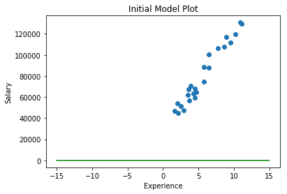
As you can see above that the green line is close to zero.This is because the initial parameters we so close to zero.

See Also

Initializing the loss function and optimizer for the regressor

We will now provide a loss function and an optimizer for out regressor. We will use Mean Squared Error for loss calculation and Stochastic Gradient Descent algorithm for optimizing and minimizing the error

#Initializing the loss function as Mean Squared Error
loss_fun = nn.MSELoss()
#Initializing the optimizer as Stochastic Gradient Descent with the model parameters and  learning rate 0.01
optimizer = torch.optim.SGD(model.parameters(), lr = 0.01)

Training the model

Finally it’s time to train our model with the training data we saved earlier. We will use a for loop to iterate through epochs or cycles of training. We will also store the losses during each cycle in a list.

# Training the model
1.epochs = 100
2.losses = []
3.for i in range(epochs):
4.    y_pred = model.forward(X_train)
5.    loss = loss_fun(y_pred, y_train)
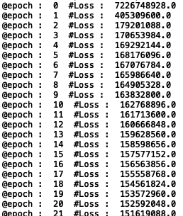
6.    print("@epoch : ", i, " #Loss : ", loss.item())
7.   losses.append(loss)
8.    optimizer.zero_grad()
9.    loss.backward()
10.    optimizer.step()

Let’s look at each line.

1. Define the number of epochs or cycles of training.Here the training will run a cycle of 50 time each time updating its weights and trying to minimize the error
2. A list for storing the losses at each cycle/epoch
3. A for loop to iterate over the epochs
4. Feeding the regressor with training data X_train
5. Passing the predicted value of X_train and actual observation to the loss function to calculate the loss
6. Printing the epoch and loss
7. Saving the loss into  a list
8. Setting the optimizer to zero gradient before backward propagation. This will help the SGD in moving the right direction of slope
9. Backpassing the losses generated at an epoch
10. Calling the step method performs a parameter update based on the current gradient and proceeds

Output:

Visualizing the loss 

#Visualizing the loss curve
plt.plot(range(epochs), losses)

Output:

From the above image image we can see a considerable decrease in loss from epochs 0 to 3. From the 3rd or 4th epochs the loss keeps almost steady. This means the model cannot further optimize itself. Now we will jump ahead and see how out trained model drew the regression line.

Visualizing the regressor after training

#Visualizing the trained regressor
plot_model("Trained Model")

Output:

From the above image, we can see that the regression line almost passes through or is closer to most of the data points. Good job. Our regressor is now officially qualified to predict Salaries for new Experiences.

Predicting Salaries for test data

#Predicting for X_test
y_pred_test = model.forward(X_test)

Comparing Actual observations and Predictions

#Converting predictions from tensor objects into a list

y_pred_test = [y_pred_test[x].item() for x in range(len(y_pred_test))]
# Comparing Actual and predicted values
df = {}
df['Actual Observation'] = y_test
df['Predicted Salary'] = y_pred_test
df = pd.DataFrame(df)
print(df)

Output:

#Visualizing Actual and predicted values
df.plot()

Output:

We can see how close the predictions are to the actual observations.Great Job !! You have created your first ever regressor in PyTorch. 

Enjoyed this story? Join our Telegram group. And be part of an engaging community.

Provide your comments below

comments